damidBind
Owen J. Marshall
Menzies Institute for Medical Research, University of Tasmaniaowen.marshall@utas.edu.au Source:
vignettes/damidBind_vignette.Rmd
damidBind_vignette.RmdAbstract
The damidBind package provides a straightforward formal analysis pipeline to analyse and explore differential DamID binding, gene transcription or chromatin accessibility between two conditions. The package imports processed data from DamID-seq experiments, either as external raw files in the form of binding bedGraphs and GFF/BED peak calls, or as internal lists of GRanges objects. After optionally normalising data, combining peaks across replicates and determining per-replicate peak occupancy, the package links bound loci to nearby genes. For RNA Polymerase DamID data, the package calculates occupancy over genes, and optionally calcualates the FDR of significantly-enriched gene occupancy. damidBind then uses either limma (for conventional log2 ratio DamID binding data) or NOIseq (for counts-based CATaDa chromatin accessibility data) to identify differentially-enriched regions, or differentially epxressed genes, between two conditions. The package provides a number of visualisation tools (volcano plots, Gene Ontology enrichment plots via ClusterProfiler and proportional Venn diagrams via BioVenn for downstream data exploration and analysis. An powerful, interactive IGV genome browser interface (powered by Shiny and igvShiny) allows users to rapidly and intuitively assess significant differentially-bound regions in their genomic context.
1 Introduction
DamID (van Steensel & Henikoff, 2000; van Steensel et al, 2001) is a highly-sensitive means to profile the genome-wide association of proteins with chromatin in living eukaryotic cells, without fixation or the use of antibodies. Cell-type specific techniques such as Targeted DamID (Southall et al, 2013; Marshall et al, 2016) to profile protein binding, and CATaDA (Aughey et al, 2018) to profile chromatin accessibility, have made the technique an extremely powerful tool to understand the binding of transcription factors, chromatin proteins, RNA polymerase and chromatin changes during development and disease.
Despite the technique’s growing popularity and adoption, no formal analysis pipeline or R package exists to analyse and explore differential DamID binding, gene transcription or chromatin accessibility between two conditions. The damidBind package provides this functionality.
damidBind imports processed data from DamID-seq experiments in the form of binding bedgraphs and GFF peak calls. After optionally normalising data, combining peaks across replicates and determining per-replicate peak occupancy, the package links bound loci to nearby genes. It then uses either limma (for conventional log2 ratio DamID binding data) or NOIseq (for counts-based CATaDa chromatin accessibility data) to identify differentially-enriched regions between two conditions. The package provides a number of visualisation tools (volcano plots, GO enrichment plots, Venn diagrams) for downstream data exploration and analysis. An interactive IGV genome browser interface (powered by Shiny and igvShiny) allows users to rapidly and intuitively assess significant differentially-bound regions.
Although extensive customisation options are available if required, much of the data handling by damidBind is taken care of automatically, with sensible defaults assumed. To move from loading raw data to visualising differentially-enriched regions on a volcano plot or browsing enriched regions in an interactive IGV window is a simple three command procedure.
2 Installation
To install from Bioconductor (stable) or github (latest), use:
if (!require("BiocManager", quietly = TRUE))
    install.packages("BiocManager")

# To install from Bioconductor (requires Bioconductor release 3.23):
BiocManager::install(version='devel')
BiocManager::install("damidBind")

# ... or to install the latest build from Github
# (requires R>4.4, should work on most recent Bioconductor releases):
BiocManager::install("marshall-lab/damidBind")
3 Quick start guide
Using damidBind, in nine easy steps:
## Example code only, not run:

# Load up the data
# (use load_data_genes() for RNA Polymerase occupancy data)
input <- load_data_peaks(
    binding_profiles_path = "path/to/binding_profile_bedgraphs",
    peaks_path = "path/to/peak_gffs_or_beds"
    # add a normalisation step via norm_method if appropriate
)

# Determine differential binding
# (use differential_accessibility() for CATaDa chromatin accessibility data)
input_diff <- differential_binding(
    input,
    cond = c(
        "Display name 1" = "Condition 1 identifying string in filenames",
        "Display name 2" = "Condition 2 identifying string in filenames"
    )
)

# The result 'input_diff' is a formal S4 object.
# You can see a summary by typing its name:
input_diff

# View the proportion of differentially bound loci
plot_venn(input_diff)

# Plot the differential binding, labelling associated genes with outliers
plot_volcano(input_diff)

# Analyse GO enrichment in peaks associated with one condition
analyse_go_enrichment(
    input_diff,
    direction = "Condition 1 identifier set with differential_binding() above"
)

# View the differentially bound loci in an Shiny/IGV browser web app,
# with an interactive, searchable, sortable table of bound regions
browse_igv_regions(input_diff)

# Apply additional functions on the differential binding results
my_custom_function(analysisTable(input_diff))

# View all analysis metadata, including genome annotation version, input files and modication times:
metadata(input_diff)
4 Sample data examples
4.1 Sample input data (provided within the package)
damidBind provides a simple, truncated dataset with the package for immediate testing. Owing to package space, this sample dataset uses only Drosophila melanogaster chromosome 2L binding, and should not be used for any actual analysis.
4.2 Sample input data (provided online through a Zenodo repository)
Three previously-published sample datasets have been deposited in Zenodo and made available for fully exploring the features and capabilities of damidBind:
- Bsh transcription factor binding in L4 and L5 neurons of the Drosophila lamina (Xu et al, 2024)
- CATaDa chromatin accessibility data in L4 and L5 neurons (Xu et al, 2024)
- RNA Polymerase II occupancy in Drosophila larval neural stem cells and adult neurons. (Marshall & Brand, 2017)
Processed files (incl. binding profiles and peaks files) are provided for all datasets.
5 Data preparation
5.1 Input data format
damidBind takes as input:
- Genome-wide binding profile tracks in bedGraph format (external files) or GenomicRanges format (internal)
- For standard DamID binding datasets, the score column is expected to be a log2 ratio
- For CATaDa chromatin accessibility datasets, the score column should be in CPM (counts per million reads) or similar
- Significant peaks files in GFF or BED format (external files) or GenomicRanges format (internal)
- Peaks are not required when comparing differential gene expression via RNA Polymerase occupancy.
All external data files are read using rtracklayer and can be gzip compressed or uncompressed as required.
5.2 Input data generation
damidBind can work with either raw data files or preprocessed data in GenomicRanges format.
5.2.1 bedGraph binding / accessibility profiles
We recommend that damidseq_pipeline is used to generate input files:
- Using default options to generate log2 ratio protein binding bedGraphs
- Using the
--catadaflag on Dam-only samples to generate count-based CATaDa accesibility bedGraphs
5.2.2 Peak GFF files
We recommend that find_peaks is used to generate peak files on each DamID / CATaDa bedGraph file replicate:
- In all cases, the default options of
--min_quant=0.8 --unified_peaks=minare recommended
6 Using damidBind
Load the library
## 6.1 Loading data
A small example dataset is provided with damidBind. The dataset is derived from the binding of Bsh in L4 and L5 neurons of the Drosophila melanogaster lamina (Xu et al, 2024), truncated to chromosome 2L. The raw data was processed using damidseq_pipeline and peaks called using find_peaks (see the publication Methods for more details).
To load up the data, we only need to know the path to the installed example datafiles:
data_dir <- system.file("extdata", package = "damidBind")

# Show the files present for clarity in this vignette example:
files <- list.files(data_dir)
print(files)
## [1] "Bsh_Dam_L4_r1-ext300-vs-Dam.kde-norm.gatc-FDR0.01.peaks.2L.bed.gz"
## [2] "Bsh_Dam_L4_r1-ext300-vs-Dam.kde-norm.gatc.2L.bedgraph.gz"
## [3] "Bsh_Dam_L4_r2-ext300-vs-Dam.kde-norm.gatc-FDR0.01.peaks.2L.bed.gz"
## [4] "Bsh_Dam_L4_r2-ext300-vs-Dam.kde-norm.gatc.2L.bedgraph.gz"
## [5] "Bsh_Dam_L5_r1-ext300-vs-Dam.kde-norm.gatc-FDR0.01.peaks.2L.bed.gz"
## [6] "Bsh_Dam_L5_r1-ext300-vs-Dam.kde-norm.gatc.2L.bedgraph.gz"
## [7] "Bsh_Dam_L5_r2-ext300-vs-Dam.kde-norm.gatc-FDR0.01.peaks.2L.bed.gz"
## [8] "Bsh_Dam_L5_r2-ext300-vs-Dam.kde-norm.gatc.2L.bedgraph.gz"And then we can use damidBind on the data. First, we load up the data. There are two potential commands that can be used for data loading, depending on the data being analysed:
load_data_peaks()-
Used to load binding data with associated peaks files (e.g. transcription factor binding, CATaDa accessibility)
load_data_genes()-
Used to load RNA Polymerase occupancy DamID data (as a proxy for gene expression, as per Marshall & Brand (2015)). For these data, no peak files are required (as occupancy is calculated over the gene bodies).
In this case, we’re dealing with the binding of the transcription factor Bsh, so we’ll use the load_data_peaks(). As this is the same transcription factor being profiled in two different cell types, and we’d expect the binding distribution to be similar, we’ll use quantile normalisation on the datasets. Other normalisation options are “loess” for limma’s cyclic LOESS normalisation; RPM (reads per million – do not use with log2 ratio data); or “none” (the default).
input.bsh <- load_data_peaks(
    binding_profiles_path = data_dir,
    peaks_path = data_dir,
    norm_method = "quantile",
    plot_diagnostics = TRUE # No need to call this in an in interactive Rstudio session:
                            # diagnostics are shown in interactive sessions by default
)
## Finding genome versions ...## Loading Ensembl genome version 'Ensembl 113 EnsDb for Drosophila melanogaster' (AH119285)## loading from cache## require("ensembldb")## Locating binding profile files## Building binding profile dataframe from input files ...## - Loaded: Bsh_Dam_L4_r1-ext300-vs-Dam.kde-norm## - Loaded: Bsh_Dam_L4_r2-ext300-vs-Dam.kde-norm## - Loaded: Bsh_Dam_L5_r1-ext300-vs-Dam.kde-norm## - Loaded: Bsh_Dam_L5_r2-ext300-vs-Dam.kde-norm## Locating peak files## Applying 'quantile' normalisation to binding profiles## Calculating occupancy over peaks## Calculating average occupancy for 1208 regions...## Generating diagnostic plots...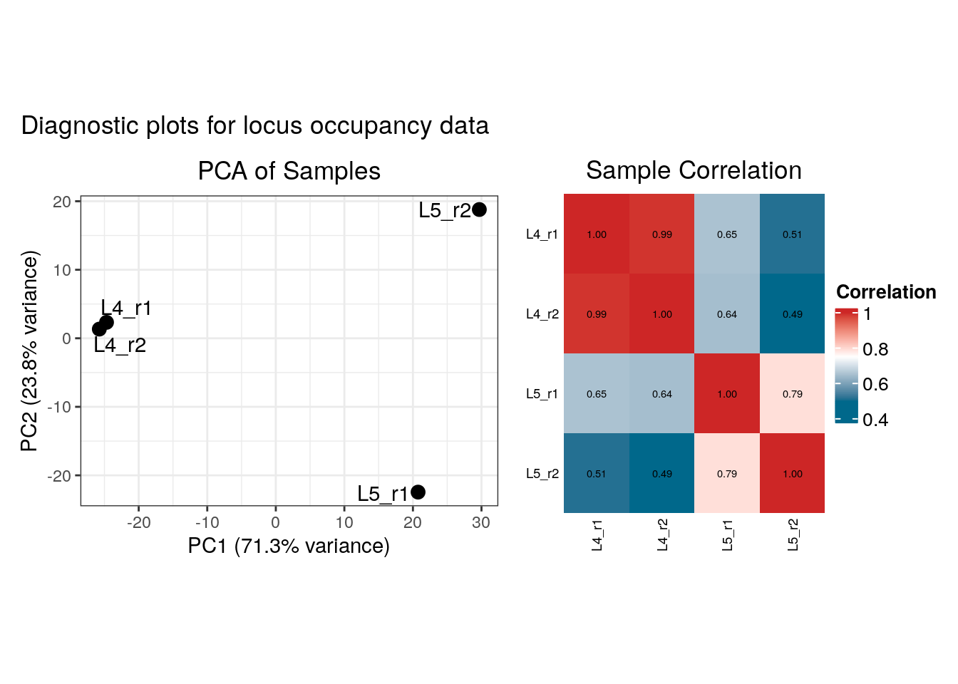
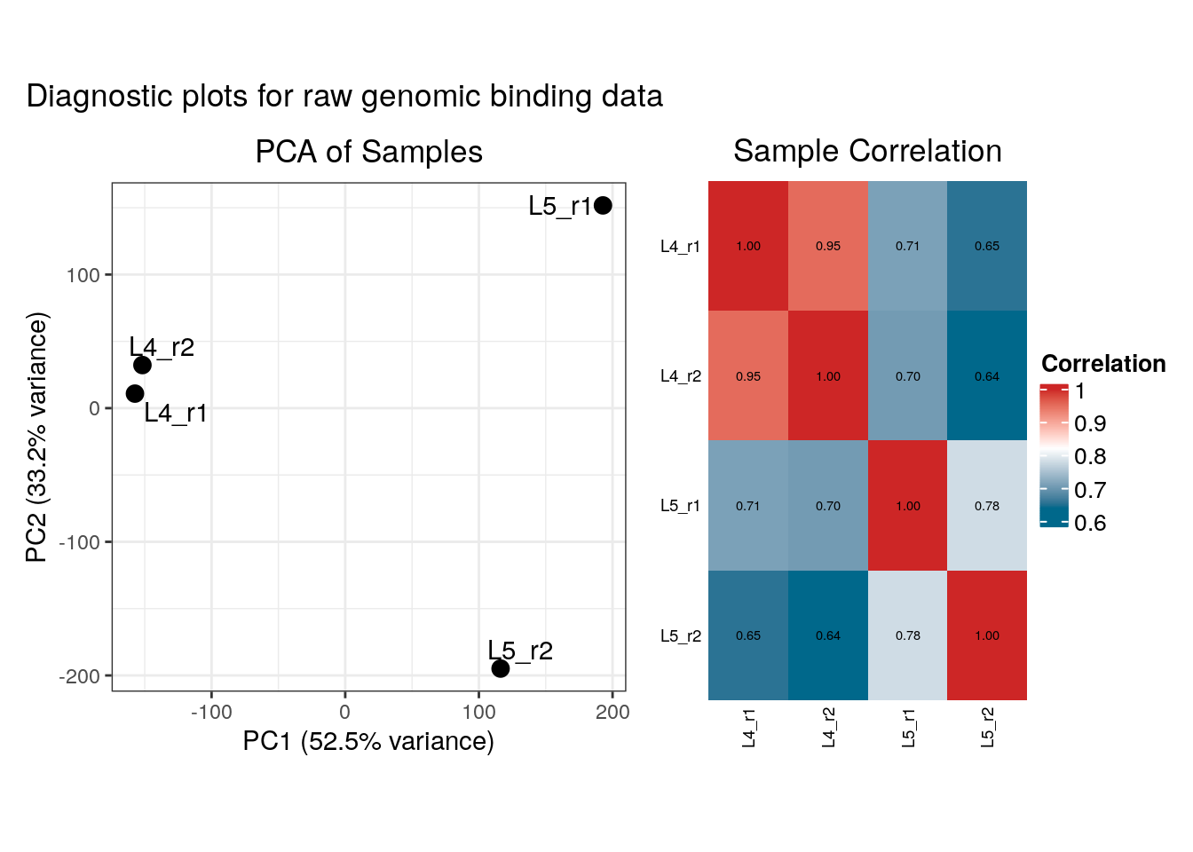
Both load_data_...functions return a diagnostics plot, illustrating a PCA plot of the samples and a clustered correlation heatmap (both for the raw genomic data and the averaged peaks). These diagnostics are displayed by default when the function in called in an interactive session, but here we use the plot_diagnostics parameter to force their display.
6.1.1 Loading data from GRanges objects
In some workflows, you may already have your binding profiles and peak regions loaded as GenomicRanges objects. damidBind supports this directly, bypassing the need to read from file paths.
The load_data_peaks() and load_data_genes() functions accept GRanges objects via the binding_profiles and peaks arguments, when used in place of binding_profiles_paths and peaks_paths. These inputs must be provided as named lists of GRanges objects, where the names correspond to your sample identifiers. For binding profiles, each GRanges object must contain exactly one numeric metadata column (e.g., score) representing the signal.
The following example first loads the provided sample data files to generate GRanges objects, and then loads these into damidBind to generate an input object ready for downstream analysis.
# Locate bedGraph and peaks example files
bedgraph_files <- list.files(data_dir, pattern = "\\.bedgraph\\.gz$", full.names = TRUE)
peak_files <- list.files(data_dir, pattern = "\\.bed\\.gz$", full.names = TRUE)

# Obtain unique sample names from the filenames (specific to these example files)
sample_names <- gsub("-ext300-vs-Dam.kde-norm.gatc.*", "", basename(bedgraph_files))

# Load the bedgraph files into a named list of GRanges objects
binding_gr_list <- lapply(bedgraph_files, rtracklayer::import)
names(binding_gr_list) <- sample_names

# Similarly, load the peak files into a named list of GRanges objects
peak_gr_list <- lapply(peak_files, rtracklayer::import)
names(peak_gr_list) <- sample_names

# Now, call load_data_peaks() using the GRanges lists instead of file paths
input.bsh_from_gr <- load_data_peaks(
    binding_profiles = binding_gr_list,
    peaks = peak_gr_list,
    norm_method = "quantile"
)
## Finding genome versions ...## Loading Ensembl genome version 'Ensembl 113 EnsDb for Drosophila melanogaster' (AH119285)## loading from cache## Building binding profile dataframe from supplied GRanges list ...## Using supplied peaks GRanges list.## Applying 'quantile' normalisation to binding profiles## Calculating occupancy over peaks## Calculating average occupancy for 1208 regions...
# The resulting object can now be used for differential analysis,
# just as in the examples below.
6.1.2 Gene locus assignment to peaks
damidBind automatically assigns peaks to genes within 1kb of the peak boundary. This value (in bp) can be changed using the maxgap_loci parameter of load_data_peaks(). Note that more than one gene locus can be assigned to a peak (especially within the gene-dense Drosophila genome).
6.1.3 A brief word on normalisation
Data normalisation for these experiments is complex, and there is no automatic solution that will work with all datasets. Avoiding normalisation with DamID-seq ratio data is often inappropriate, but incorrect normalisation can also cause issues. See the damdidBind preprint (https://doi.org/10.64898/2026.01.06.698059) for more details and a case study with the Bsh binding data. The diagnostic plots generated by damidBind should help assess normalisation outcomes, but users are also advised to carefully consider biological priors when assessing normalisation, and in particular, whether there may be asymmetry in the binding targets.
6.2 Analysing differential binding
Now, we’ll determine the differential binding of Bsh between L4 and L5 neurons. Our input files use L4 and L5 labels to distinguish the samples, and that’s all we need to know here.
Again, there are two different analysis options depending on the data type:
differential_binding()-
Analyses conventional DamID data (including RNA Polymerase DamID) present as a log2(Dam-fusion/Dam-only) ratio. All standard DamID data is in this format. limma is used as the backend for analysis.
differential_accessibility()-
Analyses CATaDa data (Dam-only chromatin accessibility data) present as Counts Per Million reads (CPM) or raw counts. Only CATaDa data (generated via e.g.
damidseq_pipeline --catada) should be used with this function. Given the counts nature of these data, NOISeq is used as the analysis backend.
The input from load_data_peaks() or load_data_genes() feeds directly into these functions.
Here, we’re not dealing with CATaDa data, so we’ll use differential_binding() to find the significant, differentially-bound loci between the two conditions:
diff.bsh <- differential_binding(
    input.bsh,
    cond = c("L4 neurons" = "L4",
             "L5 neurons" = "L5"),
    plot_diagnostics = TRUE # No need to call this in an in interactive Rstudio session:
                            # diagnostics are shown in interactive sessions by default
)
## Condition display names were sanitized for internal data:## 'L4 neurons' -> 'L4.neurons'## 'L5 neurons' -> 'L5.neurons'## Applying filter: Loci must have occupancy > 0 in at least 2 samples of at least one condition.## Filtered out 12 loci. 1196 loci remain for analysis.## Differential analysis setup:## Condition 1 Display Name: 'L4 neurons' (Internal: 'L4.neurons', Match Pattern: 'L4')## Found 2 replicates:
## Bsh_Dam_L4_r1-ext300-vs-Dam.kde-norm_qnorm
## Bsh_Dam_L4_r2-ext300-vs-Dam.kde-norm_qnorm## Condition 2 Display Name: 'L5 neurons' (Internal: 'L5.neurons', Match Pattern: 'L5')## Found 2 replicates:
## Bsh_Dam_L5_r1-ext300-vs-Dam.kde-norm_qnorm
## Bsh_Dam_L5_r2-ext300-vs-Dam.kde-norm_qnorm## limma contrasts: L4.neurons-L5.neurons## Applying eBayes moderation with `trend = TRUE, robust = TRUE`##
## Filtering for positive enrichment (mean score > 0 in the enriched condition).##
## 316 loci enriched in L4 neurons## Highest-ranked genes:
## oaf,Slh, MICU1, CG12194,tank, GramD1B, CG11927,mxt, tutl, CG17490,lncRNA:CR46268,RpL5,snoRNA:Psi28S-2996, CG4972,Usp14, La,RtGEF,snoRNA:Me28S-A3365, gcm2,Trx-2##
## 166 loci enriched in L5 neurons## Highest-ranked genes:
## beat-Ic, CG13946, CG11634, Ance-3, Ccdc85, Ugt36F1, dmGlut,lncRNA:CR44587, osp, CG42750, CG10237## Displaying diagnostic plots...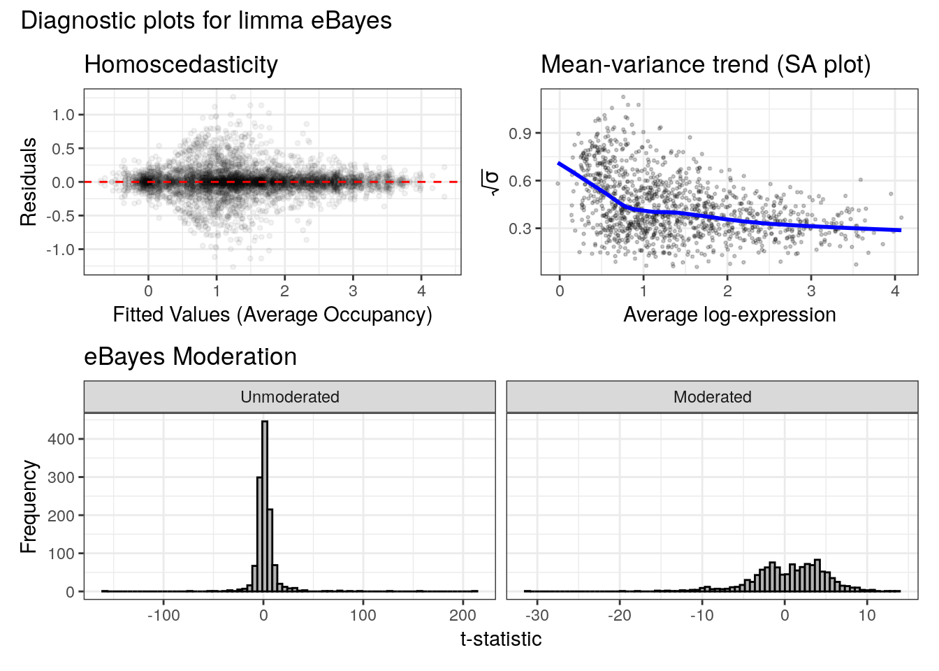
Note the required cond parameter to this function, which specifies the filename text that distinguished the two separate conditions to test. cond[1] must be a text string present in all, and only all, of the filenames of the first condition to test; cond[2] must be a text string present in all, and only all, of the filenames of the second condition to test. The vector is typically a named vector, where the names are the display names to use in plots, but providing a named vector is optional.
When run, differential_binding (or differential_accessibility) will list the replicates found under each condition. The package attempts to ensure that condition search overlaps are avoided, but please check that all replicates have been correctly assigned.
The functions’ output provides a quick “top ten” list of genes associated with the most significant, differentially bound loci. This is provided for a quick verification that the analysis has worked correctly, and does not imply any special value to the listed genes beyond that.
When calling the limma-based differential_binding() function, a diagnostic plot is also displayed illustrating the ability of limma’s empirical Bayes moderation to fit the data. differential_accessibility(), which uses the non-parametric NOISeq analysis, does not display diagnostics.
Both differential_binding() and differential_accessibility() return a DamIDResults S4 object, that forms the basis of downstream analysis. Printing the object will provide a simple summary of the analysis results.
# See a summary of the results object
diff.bsh
## An object of class 'DamIDResults'
## Differentially bound regions
## Comparison: 'L4 neurons' vs 'L5 neurons'
## - 316 regions enriched in L4 neurons
## - 166 regions enriched in L5 neurons
## - 1196 total regions tested
##
## Data provenance:
## - Annotation: drosophila_melanogaster (BDGP6.46, AH119285, Ensembl 113)
## - Data: 4 binding profile(s), 4 peak file(s)To fully explore the differentially bound loci, use one of the visualisation functions below.
6.3 Analysing differential expression
The sample dataset provided is a transcription factor binding dataset, with pre-called peaks. If analysing gene expression datasets via RNA Polymerase DamID and load_data_genes(), the analysis pipeline is similar, with some exceptions:
- No peaks are required. damidBind calculates signal occupancy over genes directly, and all downstream analyses are conducted on gene loci.
- Optional FDR calling via
load_data_genes(calculate_occupancy_pvals = TRUE). damidBind can determine the FDR for enriched occupancy of RNA Polymerase over gene bodies, which we have previously shown to be a proxy for gene expression (Southall et al, 2013; Marshall et al, 2016). - FDR values are not used for DEG analysis, but when present these can and should be used to filter the Venn and volcano plot outputs via the
fdr_filter_thresholdparameter, so that only genes deemed to be expressed are shown. - The accessor method
expressed()provides a quick means to obtain the list of genes passing an FDR threshold for one of the analysed conditions.
6.4 Visualising data
All downstream visualisation / data exploration functions take the DamIDResults object returned from the analysis functions differential_binding() or differential_accessibility().
6.4.1 Venn diagrams of differentially bound loci
Venn diagrams are a simple means of visualising the proportion of loci that are differentially bound between the two tested conditions. To provide this, damidBind uses BioVenn to generate proportional Venn diagrams of the two conditions (Figure 6.1). The set union represents significant binding peaks that fail to show significant differences in occupancy; the exclusive regions of each set represent regions with enriched differential binding in that condition.
plot_venn(diff.bsh)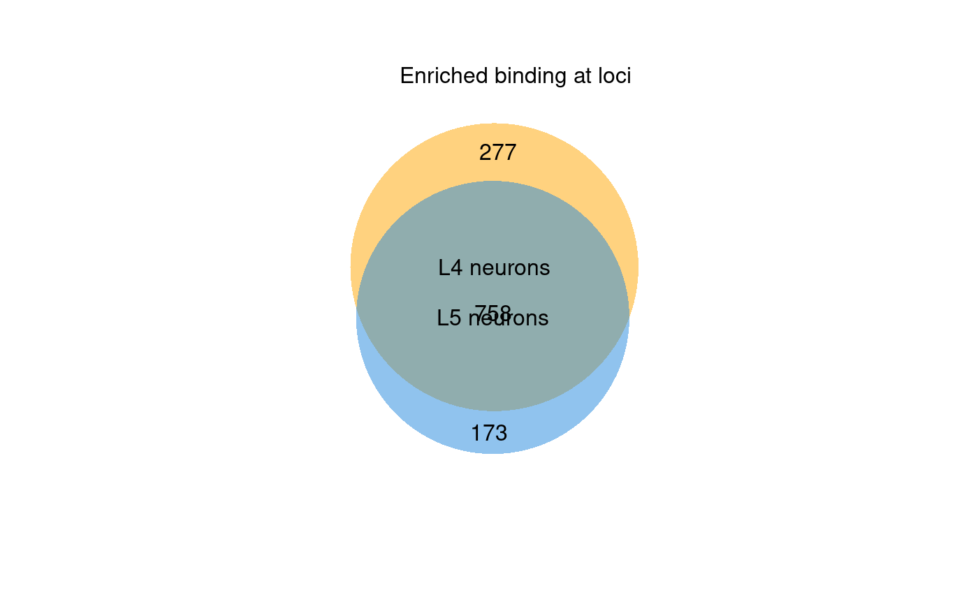
Figure 6.1: A venn diagram of significantly bound loci by Bsh in L4 and L5 neurons. The exclusive parts of each set represent regions that are differentially bound between the two conditions.
6.4.2 Volcano plots
damidBind comes with a comprehensive volcano plot function. The following gives some idea as to the capabilities.
6.4.2.1 The default volcano plot
The simple volcano plot already gives a clear picture of differentially bound loci and their associated genes (Figure 6.2).
plot_volcano(
    diff.bsh
)
## Label sampling: coordinates have been centred and scaled.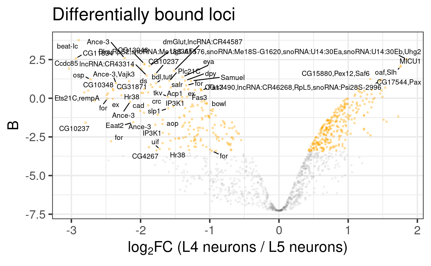
Figure 6.2: Differential binding of Bsh in L4 and L5 neuronal subtypes. Genes associated with differentially bound peaks are displayed; the limitations of label overlaps means that only outliers are labelled. (Dataset from chromosome 2L only)
6.4.2.2 Cleaning up the gene names
However, a lot of plot label space can be taken up by generally uninformative snoRNA / tRNA genes. We can optionally remove these from the plot using the clean_names=TRUE parameter, to show more potentially informative labels (Figure 6.3).
plot_volcano(
    diff.bsh,
    label_config = list(clean_names = TRUE)
)
## Label sampling: coordinates have been centred and scaled.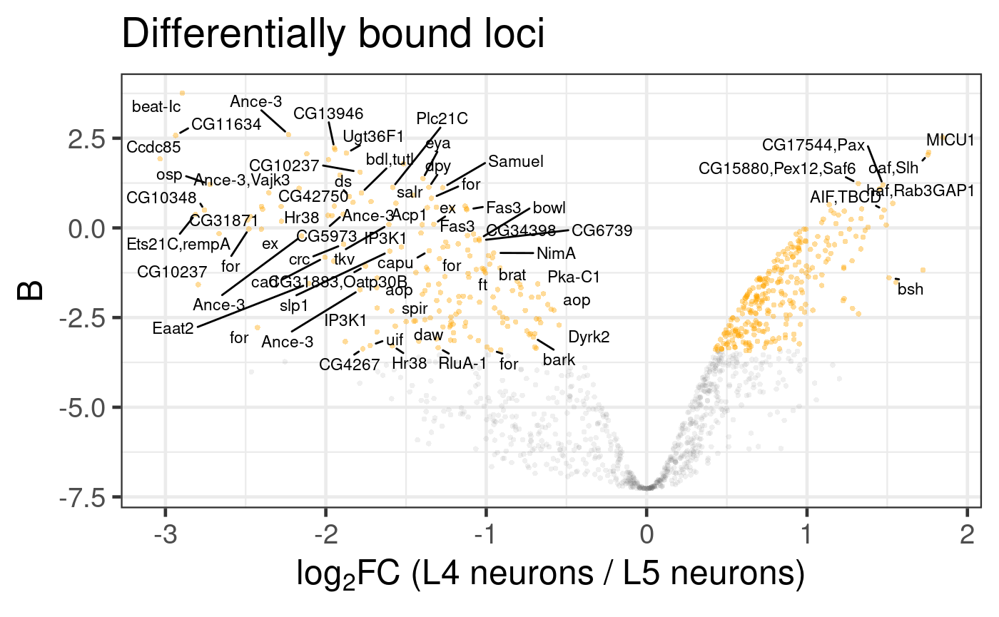
Figure 6.3: Differential binding of Bsh in L4 and L5 neuronal subtypes. Genes associated with differentially bound peaks are displayed, after some common, but less useful, gene label classes are removed. (Dataset from chromosome 2L only)
Already, that’s becoming a lot clearer.
Note that not every locus will get a label when the loci density is high, as there simply is not room to fit all the labels in. damidBind tries to maximise the number of labels even within dense regions, and the label_config and label_display parameter list options to plot_volcano provide additional configuration options to allow any plot labels to be optimised.
6.4.2.3 Highlighting gene groups
But, what if we now wanted to highlight genes bound by Bsh, that are only expressed in L4 neurons? (data from scRNA-seq data, provided in Supplementary Files 2 & 3 of (Xu et al, 2024)). This is straightforward to do (Figure 6.4).
L4_only_genes <- c("Mp", "tnc", "grn", "rut", "mtd", "rdgB", "Octbeta2R", "msi", "Octbeta3R", "beat-IIIb", "ap", "Fili", "LRP1", "CG7378", "CG13698", "twit", "CG9336", "tok", "CG12991", "dpr1", "CG42339", "beat-IIb", "mav", "CG34377", "alpha-Man-IIb", "Pli", "CG32428", "osp", "Pka-R2", "CG15202", "CG8916", "CG15894", "side", "CG42258", "CHES-1-like", "SP2353", "CG44838", "Atg1", "Traf4", "DIP-beta", "KCNQ", "metro", "nAChRalpha1", "path", "CG10527", "Pde8", "CG30116", "CG7985", "CG1688", "dpr12", "pigs", "Eip63F-1", "CG14795", "2mit", "CG42340", "BicD", "CG18265", "hppy", "5-HT1A", "Chd64", "CG33090", "Dyb", "Btk29A", "Apc", "Rox8", "nAChRalpha5", "CG42748", "CG3257", "CG2269", "beat-IV", "CG8086", "glec", "CG31688", "oaf", "Drl-2", "CG8188", "aos", "CG31676", "REPTOR", "RabX4", "alt", "Pura", "DIP1", "ewg", "side-VIII", "nAChRalpha7", "Alh", "kug", "Ca-Ma2d", "bru2", "CG43737", "lncRNA:CR44024", "lncRNA:CR46006", "Had1", "CG3961", "comm", "Toll-6", "CG13685", "tow", "CG10019")

plot_volcano(
    diff.bsh,
    label_config = NULL,
    highlight = list(
        "L4 specific" = L4_only_genes
    ),
    highlight_config = list(
        size = 2
    )
)
## Label sampling: too few points to effectively sample; all will be labelled.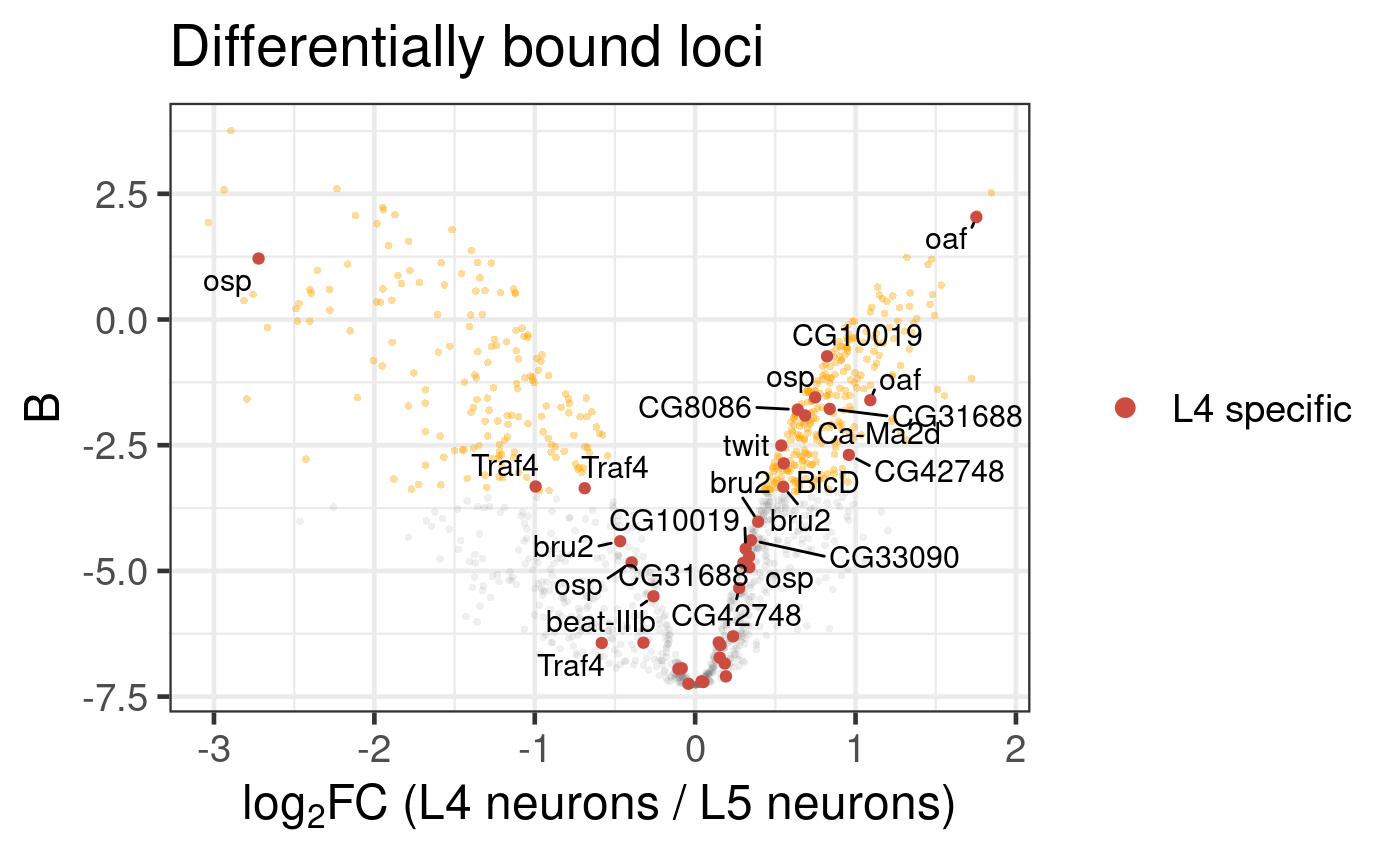
Figure 6.4: Differential binding of Bsh in L4 and L5 neuronal subtypes. Genes that are specifically expressed in L4 neurons are highlighted. (Dataset from chromosome 2L only)
Note that the legend guide masks some labels, when positioned inside the plot on the right-hand side (the default). damidBind comes with a simple shortcut to display the legend on the left side of the plot instead (highlight_config = list(legend_inside_pos = 'l')), as shown below (Figure 6.5). It is also possible to place the legend outside the plot, or to customise the position of the legend within the plot precisely.
plot_volcano(
    diff.bsh,
    label_config = NULL,
    highlight = list(
        "L4 specific" = L4_only_genes
    ),
    highlight_config = list(
        size = 2,
        legend_inside_pos = 'l'
    )
)
## Label sampling: too few points to effectively sample; all will be labelled.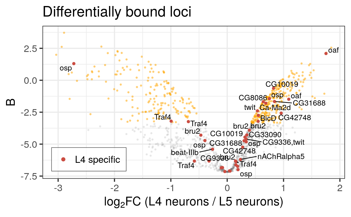
Figure 6.5: Differential binding of Bsh in L4 and L5 neuronal subtypes. Genes that are specifically expressed in L4 neurons are highlighted. (Dataset from chromosome 2L only). Legend is now displayed on the LHS within the plot.
Although this is just a truncated sample from chr 2L, the link between a subset of Bsh binding and potential upregulation in this lineage is apparent. (Why do some gene loci label multiple peaks? This is because a gene may have more than one discrete binding peak associated with it.)
We could also compare this against genes bound by Bsh and only expressed in L5 neurons. For clarity, we’ll colour the text labels to match the conditions, and we’ll reduce the text luminosity to make the labels easier to read (Figure 6.6).
L5_only_genes <- c("Ptth", "Nep2", "kek1", "CG4168", "kek3", "CG6959", "Dtg", "ND-23", "Scp2", "Octalpha2R", "Hs6st", "CG16791", "SKIP", "LpR1", "RpL34a", "Ald1", "CG10011", "heph", "nolo", "Act42A", "Fkbp12", "Pkc53E", "AstC-R1", "Muc14A", "CG33543", "ChAT", "Act5C", "Ptpmeg2", "fabp", "CG31221", "Octbeta1R", "CG14669", "sdk", "Shawl", "side-V", "NaCP60E", "sif", "OtopLc", "side-II", "kuz", "CG42540", "Dscam3", "haf", "CG42673", "pdm3", "tinc", "CG42750", "sdt", "Nuak1", "Hk", "scrib", "tsr", "dpr20", "GluRIB", "CG43902", "CG44242", "Dscam2", "CG44422", "lncRNA:CR45312", "Scsalpha1", "Rop", "Con", "Hsc70-3", "dpr8", "eag", "ND-18", "Nrt", "CG17839", "fz", "CG32137", "Rh7", "Sod1", "CG32052", "dpr6", "Hsp67Ba", "axed", "GluRIA", "robo2")


plot_volcano(
    diff.bsh,
    label_config = NULL,
    highlight = list(
        "L4 specific" = L4_only_genes,
        "L5 specific" = L5_only_genes
    ),
    highlight_config = list(
        size = 2,
        legend_inside_pos = 'l',
        text_col = TRUE,
        text_luminosity = 40
    )
)
## Label sampling: too few points to effectively sample; all will be labelled.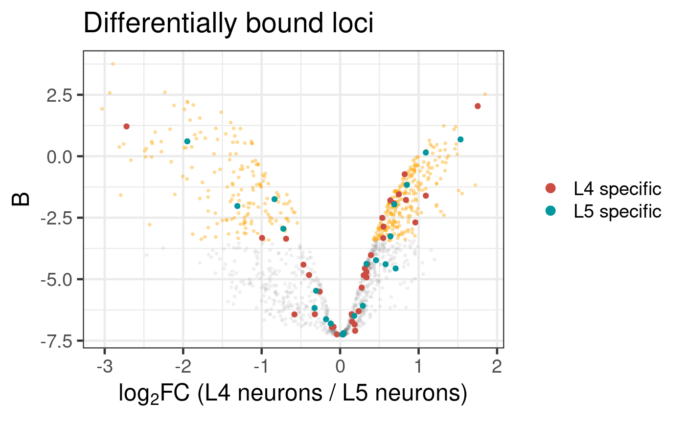
Figure 6.6: Differential binding of Bsh in L4 and L5 neuronal subtypes. Genes that are specifically expressed in each subtype are highlighted. (Dataset from chromosome 2L only)
Here, the L5-specific Bsh peaks show no clear link with upregulated or downregulated genes between the lineages.
6.4.3 Browsing differentially-bound regions
A volcano plot, while useful, still does not put the binding data into a genomic context. For this damidBind provides an interactive Shiny browser window (via Shiny and igvShiny), where an interactive table of enriched loci allows quick exploration of these in the genome browser.
## Interactive, blocking session, uncomment to run
# browse_igv_regions(diff.bsh)
An example of the interface is shown below (Figure 6.7).
Figure 6.7: The interactive IGV browser window. The interface allows for rapid exploration of differentially bound regions in their genomic context. The table of significant loci is interactive and controls the genome browser view.
The table on the left side of the window can be sorted by clicking on the column headers, and clicking on any entry will move the IGV browser window to that locus (+/- a sensible buffer region). All sample reps are shown, together with the unified binding peaks and a simple pair of tracks that show the loci that are enriched in both conditions.
The default display will show the individual replicate tracks. In order to show the averaged binding per condition instead, set average_tracks = TRUE.
While this web app will save high quality SVGs, if you wish to generate your own genome browser figures with another utility, calling browse_igv_regions() with export_data_archive = "a/valid/filepath.zip" will export all of the final processed data tracks (including unified peaks and enrichment tracks) as a zip file. These can be loaded into any third party software, such as pyGenomeTracks.
The export_data_archive parameter can be combined with average_tracks = TRUE to export averaged genome-wide binding tracks.
6.4.4 Gene Ontology (GO) enrichment plots
Gene ontology is a powerful means of understanding which biological processes may be changing between two sets of data. Using clusterProfiler as the backend, damidBind provides the function analyse_go_enrichment() to explore enrichment of genes associated with bound peaks, accessible regions, or differential expression. In all cases, the underlying gene IDs, rather than gene names, are used for enrichment analysis.
The example dataset here is minimal, so there is not much to highlight when we look at just the genes enriched in close proximity to L5-specific binding peaks (Figure 6.8).
go.bsh_l4 <- analyse_go_enrichment(
    diff.bsh,
    direction = "L5",
    org_db = org.Dm.eg.db::org.Dm.eg.db
)
## 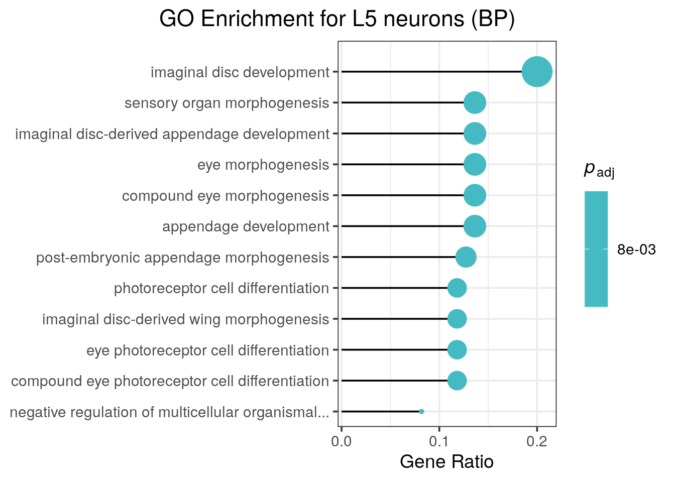
Figure 6.8: Enriched GO terms for genes associated with differential Bsh binding in L5 neuron. Dataset from chromosome 2L only.
The return value of this function includes the full analysis table, including the names of all enriched loci within an ontology term.
6.5 Accessor methods and further analysis
The DamIDResults object returned by differential_binding() and differential_accessibility() provides accessor methods for accessing data for further analysis.
The following accessor functions are available for a DamIDResults object.
-
analysisTable(object): Returns the full differential analysis table (adata.frame). -
enrichedCond1(object): Returns adata.frameof regions significantly enriched in the first condition. -
enrichedCond2(object): Returns adata.frameof regions significantly enriched in the second condition. -
conditionNames(object): Returns a named character vector mapping display names to internal identifiers. -
inputData(object): Returns a list containing the original input data used for the analysis. -
expressed(object, condition, fdr = 0.05, which = "any"): Returns adata.frameof genes considered expressed in ‘condition’, based on an FDR threshold of significantly enriched occupancy. Only available for analyses with FDR calculations, generated viaload_data_genes(calculate_occupancy_pvals = TRUE). -
metadata(object): Returns all input file and genome annotation metadata.
7 References
8 Session info
## R version 4.4.0 (2024-04-24)
## Platform: x86_64-pc-linux-gnu
## Running under: Ubuntu 22.04.5 LTS
##
## Matrix products: default
## BLAS:   /usr/lib/x86_64-linux-gnu/openblas-pthread/libblas.so.3
## LAPACK: /usr/lib/x86_64-linux-gnu/openblas-pthread/libopenblasp-r0.3.20.so;  LAPACK version 3.10.0
##
## locale:
##  [1] LC_CTYPE=en_AU.UTF-8       LC_NUMERIC=C
##  [3] LC_TIME=en_AU.UTF-8        LC_COLLATE=en_AU.UTF-8
##  [5] LC_MONETARY=en_AU.UTF-8    LC_MESSAGES=en_AU.UTF-8
##  [7] LC_PAPER=en_AU.UTF-8       LC_NAME=C
##  [9] LC_ADDRESS=C               LC_TELEPHONE=C
## [11] LC_MEASUREMENT=en_AU.UTF-8 LC_IDENTIFICATION=C
##
## time zone: Etc/UTC
## tzcode source: system (glibc)
##
## attached base packages:
## [1] stats4    stats     graphics  grDevices utils     datasets  methods
## [8] base
##
## other attached packages:
##  [1] ensembldb_2.30.0        AnnotationFilter_1.30.0 GenomicFeatures_1.58.0
##  [4] AnnotationDbi_1.68.0    Biobase_2.66.0          GenomicRanges_1.58.0
##  [7] GenomeInfoDb_1.42.3     IRanges_2.40.1          S4Vectors_0.44.0
## [10] BiocGenerics_0.52.0     damidBind_1.1.1         BiocStyle_2.34.0
##
## loaded via a namespace (and not attached):
##   [1] splines_4.4.0               later_1.4.4
##   [3] BiocIO_1.16.0               bitops_1.0-9
##   [5] ggplotify_0.1.3             filelock_1.0.3
##   [7] tibble_3.3.0                R.oo_1.27.1
##   [9] XML_3.99-0.19               lifecycle_1.0.4
##  [11] httr2_1.2.1                 org.Dm.eg.db_3.20.0
##  [13] doParallel_1.0.17           lattice_0.22-7
##  [15] backports_1.5.0             NOISeq_2.50.0
##  [17] magrittr_2.0.4              limma_3.62.2
##  [19] sass_0.4.10                 rmarkdown_2.30
##  [21] jquerylib_0.1.4             yaml_2.3.10
##  [23] plotrix_3.8-4               otel_0.2.0
##  [25] httpuv_1.6.16               ggtangle_0.0.7
##  [27] cowplot_1.2.0               DBI_1.2.3
##  [29] RColorBrewer_1.1-3          abind_1.4-8
##  [31] zlibbioc_1.52.0             Rtsne_0.17
##  [33] purrr_1.1.0                 R.utils_2.13.0
##  [35] RCurl_1.98-1.17             yulab.utils_0.2.1
##  [37] rappdirs_0.3.3              circlize_0.4.16
##  [39] GenomeInfoDbData_1.2.13     enrichplot_1.26.6
##  [41] ggrepel_0.9.6               tidytree_0.4.6
##  [43] svglite_2.2.2               codetools_0.2-20
##  [45] DelayedArray_0.32.0         DOSE_4.0.1
##  [47] DT_0.34.0                   xml2_1.4.1
##  [49] shape_1.4.6.1               tidyselect_1.2.1
##  [51] futile.logger_1.4.3         aplot_0.2.9
##  [53] UCSC.utils_1.2.0            farver_2.1.2
##  [55] matrixStats_1.5.0           BiocFileCache_2.14.0
##  [57] GenomicAlignments_1.42.0    jsonlite_2.0.0
##  [59] GetoptLong_1.0.5            iterators_1.0.14
##  [61] randomcoloR_1.1.0.1         systemfonts_1.3.1
##  [63] foreach_1.5.2               dbscan_1.2.3
##  [65] tools_4.4.0                 ggnewscale_0.5.2
##  [67] progress_1.2.3              treeio_1.30.0
##  [69] Rcpp_1.1.0                  glue_1.8.0
##  [71] SparseArray_1.6.2           mgcv_1.9-3
##  [73] xfun_0.54                   qvalue_2.38.0
##  [75] MatrixGenerics_1.18.1       dplyr_1.1.4
##  [77] withr_3.0.2                 formatR_1.14
##  [79] BiocManager_1.30.26         fastmap_1.2.0
##  [81] digest_0.6.37               BioVenn_1.1.3
##  [83] mime_0.13                   R6_2.6.1
##  [85] gridGraphics_0.5-1          textshaping_1.0.4
##  [87] colorspace_2.1-2            GO.db_3.20.0
##  [89] biomaRt_2.62.1              RSQLite_2.4.3
##  [91] R.methodsS3_1.8.2           tidyr_1.3.1
##  [93] generics_0.1.4              data.table_1.17.8
##  [95] rtracklayer_1.66.0          prettyunits_1.2.0
##  [97] httr_1.4.7                  htmlwidgets_1.6.4
##  [99] S4Arrays_1.6.0              pkgconfig_2.0.3
## [101] gtable_0.3.6                blob_1.2.4
## [103] ComplexHeatmap_2.22.0       S7_0.2.0
## [105] XVector_0.46.0              clusterProfiler_4.14.6
## [107] htmltools_0.5.8.1           bookdown_0.45
## [109] fgsea_1.32.4                clue_0.3-66
## [111] ProtGenerics_1.38.0         scales_1.4.0
## [113] png_0.1-8                   ggfun_0.2.0
## [115] lambda.r_1.2.4              knitr_1.50
## [117] rstudioapi_0.17.1           reshape2_1.4.4
## [119] rjson_0.2.23                checkmate_2.3.3
## [121] nlme_3.1-168                curl_7.0.0
## [123] GlobalOptions_0.1.2         cachem_1.1.0
## [125] stringr_1.5.2               BiocVersion_3.20.0
## [127] parallel_4.4.0              restfulr_0.0.16
## [129] pillar_1.11.1               grid_4.4.0
## [131] vctrs_0.6.5                 promises_1.5.0
## [133] dbplyr_2.5.1                cluster_2.1.8.1
## [135] xtable_1.8-4                evaluate_1.0.5
## [137] magick_2.9.0                futile.options_1.0.1
## [139] cli_3.6.5                   compiler_4.4.0
## [141] Rsamtools_2.22.0            rlang_1.1.6
## [143] crayon_1.5.3                igvShiny_1.2.0
## [145] labeling_0.4.3              plyr_1.8.9
## [147] forcats_1.0.1               fs_1.6.6
## [149] stringi_1.8.7               BiocParallel_1.40.2
## [151] Biostrings_2.74.1           lazyeval_0.2.2
## [153] V8_8.0.1                    GOSemSim_2.32.0
## [155] Matrix_1.7-4                hms_1.1.4
## [157] patchwork_1.3.2             bit64_4.6.0-1
## [159] ggplot2_4.0.0               KEGGREST_1.46.0
## [161] statmod_1.5.1               shiny_1.11.1
## [163] SummarizedExperiment_1.36.0 AnnotationHub_3.14.0
## [165] igraph_2.2.1                memoise_2.0.1
## [167] bslib_0.9.0                 ggtree_3.12.0
## [169] fastmatch_1.1-6             bit_4.6.0
## [171] ape_5.8-1                   gson_0.1.0